Eigenvectors and communities
I liked a lot the talk by Luca Trevisan in STOC’09 about the “Max Cut and the Smallest Eigenvalue”. In this paper he proposes an -approximation algorithm for MAX-CUT, which is the first approximation algorithm for MAX-CUT that doesn’t use semi-definite programming (SDP). The best possible approximation for that problem is the 0.878-approximation given by Goemans and Williamson, based on SDP (which is the best possible approximation assuming the Unique Games Conjecture).
I won’t discuss the paper in much detail here, but its heart is the very beautiful idea of analyzing properties of a graph looking at the spectrum of the matrix that defines it. For example, represent a graph by its adjacent matrix
, i.e.,
is an
matrix (where
is the number of nodes of
) and
iff the edge
is in
. Let also
be the diagonal matrix for which
is the degree of node
. The normalized adjacency matrix is given by
. Let
be its eigenvalues. It is easy to see that all the eigenvalues are in
, since:
taking we have that:
for all
. It is not hard to see the the maximum eigenvalue is:
To prove it is analogous, just by analyzing
. The next natural questions is: do those bounds hold with equality?
In fact, for all graphs. It is very easy to see that, just take the vector
with
where
is the degree of node
. And for
, it is not difficult to see that
iff the graph has a bipartite connected component. It is also easy to see that if the graph has
connected components then
.
So, given a connected graph . But what happens if
is very close to
. Intuitively, it means that the graph is almost disconnected in the sense that it has a very sparse cut. For
-regular graphs (a graph where all nodes have degree
), this intuition is captured by Cheeger’s inequality.
where is the sparsity of
, defined as
. In the paper, Luca Trevisan discusses an analogue os Cheeger’s Inequality for the smallest eigenvalues
. Instead of measuring how close we are from a disconnected graph, we measure how close we are from a a bipartite graph.
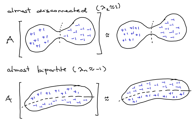
Let’s try to get some intuition: if a -regular graph has a good sparse cut, like in the picture below, we could divide it in two parts and try to get an eigenvalue close to
by the following way: set “almost”
in one part and almost
in the other. Since there are very few edges crossing the cut, after being transformed by
the values are almost still the same. Also if the graph is almost bipartite, we can set almost
in one part and almost
in the other, and after applying
, what was
becomes
and vice versa.

Ok, we can use eigenvalues to have a good idea if the graph has good expansion or not, but how to use that to actually find good partitions of it? Let be the eigenvector corresponding to
. The intuition in the last paragraph tells us that maybe we should think of getting
and
. More generally we can substitute
by a threshold
. This gives us only
possible partitions to test and choose the best, instead of
.
Finding Communities in Graphs
Real world graphs like social networks have clusters of nodes that can be identified as communities. There is a lot of work in finding those communities using all sorts of methods – more references about that can be found in Jon Kleinberg’s Networks course website. Spectral techniques are a natural candidate for doing that. I did a small experiment using Orkut, the most used social network in Brasil. Let be the entire graph of Orkut and
be the node representing my profile on
and let:
be the set of all my friends and
be the graph induced on my friends.
First, I crawled the web to reconstruct (notice I am not in the graph, so I am not using the fact that I am connecting all them. I am just using the connections between them). First, I have
friends, which form a huge
nodes component, and smaller components (one of size
, two of size
and six of size
). Let’s forget about the smaller components and care about the huge component: in this component there are my friends from undergrad, my friends from high-school, my family and some miscellaneous friends. Although all of them are interconnected, I wanted to be able to separate them just by using the topology of the graph.
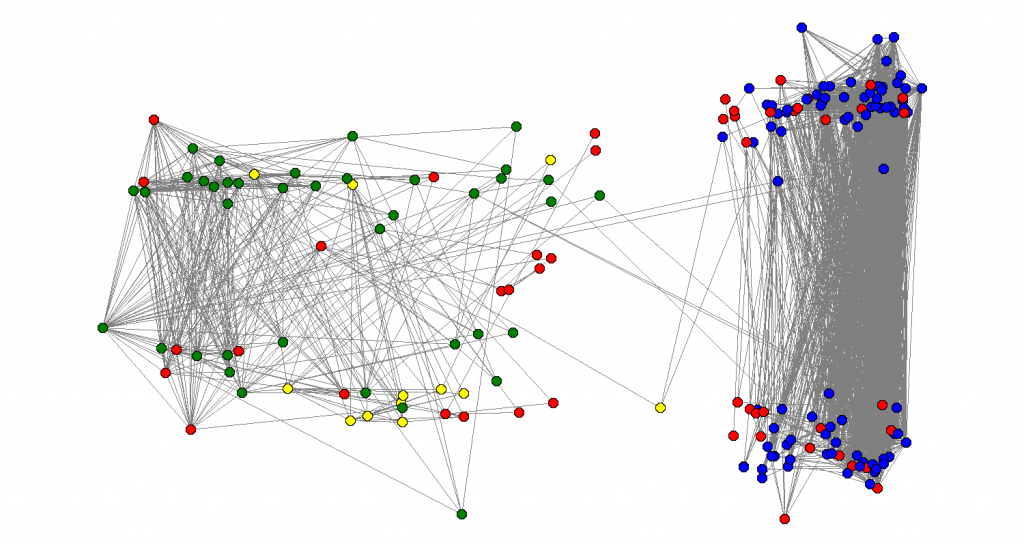
I did the following experiment: I calculated the eigenvalues and eigenvectors of . Let
be the eigenvalues and
be the eigenvectors. For each node
, I associated with coordinates
in a way that a vertical cut would be a good approximation of the sparsest cut and an horizontal line would be a good approximation of the max-cut. The result is there:

After doing that I labeled the nodes of the graph with colors: my friends from IME (my undergrad university), I labeled blue. My friends from high-school, I labeled green, my family nodes, I labeled yellow and friends from other places, I labeled red. Also, there were some people that used strange characters in their names I could no parse, so I also labeled them red. I was happy to see that the algorithm efficiently separated the green from the blue nodes: clearly distinguishing between my high-school and my undergrad friends.
More about spectral methods
Luca Trevisan has a lot of very cool blog posts about Cheeger’s inequality and other interesting proofs of spectral facts. This MIT course has a lot of material about Spectral Graph Theory.
Thanks!
Helps a lot.
Thank you for some other fantastic article. Where else may anyone get that type of info in such an ideal manner of writing? I’ve a presentation subsequent week, and I am on the look for such info.