Big Red Bits

Today in a dinner with Thanh, Hu and Joel I heard about a paradox I haven’t heard so far. Probability is full of cute problems that challenge our understanding of the basic concepts. The most famous of them is the Monty Hall Problem, which asks:

You are on a TV game show and there are doors – one of them contains a prize, say a car and the other two door contain things you don’t care about, say goats. You choose a door. Then the TV host, who knows where the prize is, opens one door you haven’t chosen and that he knows has a goat. Then he asks if you want to stick to the door you have chosen or if you want to change to the other door. What should you do?

Probably you’ve already came across this question in some moment of your life and the answer is that changing doors would double your probability of getting the price. There are several ways of convincing your intuitions:

• Do the math: when you chose the door, there were three options so the prize is in the door you chose with probability and in the other door with probability (note that the presenter can always open some door with a goat, so conditioning on that event doesn’t give you any new information).
• Do the actual experiment (computationally) as done here. One can always ask a friend to help, get some goats and perform the actual experiment.
• To convince yourself that “it doesn’t matter” is not correct, think doors. You choose one and the TV host open of them and asks if you want to change or stick with your first choice. Wouldn’t you change?

I’ve seen TV shows where this happened and I acknowledge that other things may be involved: there might be behavioral and psychologic issues associated with the Monty Hall problem – and possibly those would interest Dan Ariely, whose book I began reading today – and looks quite fun. But the problem they told me about today in dinner was another: the envelope problem:

There are two envelopes and you are told that in one of them there is twice the amount that there is in the other. You choose one of the envelopes at random and open it: it contains bucks. Now, you don’t know if the other envelope has bucks or bucks. Then someone asks you if you wanted to pay bucks and change to the other envelope. Should you change?

Now, consider two different solutions to this problem: the first is fallacious and the second is correct:

1. If I don’t change, I get bucks, if I change I pay a penalty of and I get either or with equal probability, so my expected prize if I change is , so I should change.
2. I know there is one envelope with and one with , then my expected prize if I don’t change is . If I change, my expected prize is , so I should not change.

The fallacy in the first argument is perceiving a probability distribution where there is no one. Either the other envelope contains bucks or it contains bucks – we just don’t know, but there is no probability distribution there – it is a deterministic choice by the game designer. Most of those paradoxes are a result of either an ill-defined probability space, as Bertrand’s Paradox or a wrong comprehension of the probability space, as in Monty Hall or in several paradoxes exploring the same idea as: Three Prisioners, Sleeping Beauty, Boy or Girl Paradox, …

There was very recently a thrilling discussion about a variant on the envelope paradox in the xkcd blag – which is the blog accompaning that amazing webcomic. There was a recent blog post with a very intriguing problem. A better idea is to go there and read the discussion, but if you are not doing so, let me summarize it here. The problem is:

There are two envelopes containing each of them a distinct real number. You pick one envelope at random, open it and see the number, then you are asked to guess if the number in the other envelope is larger or smaller then the previous one. Can you guess correctly with more than probability?

A related problem is: given that you are playing the envelope game and there are number and (with ). You pick one envelope at random and then you are able to look at the content of the first envelope you open and then decide to switch or not. Is there a strategy that gives you expected earnings greater than ?

The very unexpected answers is yes !!! The strategy that Randall presents in the blog and there is a link to the source here is: let be a random variable on such that for each we have , for example, the normal distribution or the logistic distribution.

Sample then open the envelope and find a number now, if say the other number is lower and if say the other number is higher. You get it right with probability

which is impressive. If you follow your guess, your expected earning is:

The xkcd pointed to this cool archive of puzzles and riddles. I was also told that the xkcd puzzle forum is also a source of excellent puzzles, as this:

You are the most eligible bachelor in the kingdom, and as such the King has invited you to his castle so that you may choose one of his three daughters to marry. The eldest princess is honest and always tells the truth. The youngest princess is dishonest and always lies. The middle princess is mischievous and tells the truth sometimes and lies the rest of the time. As you will be forever married to one of the princesses, you want to marry the eldest (truth-teller) or the youngest (liar) because at least you know where you stand with them. The problem is that you cannot tell which sister is which just by their appearance, and the King will only grant you ONE yes or no question which you may only address to ONE of the sisters. What yes or no question can you ask which will ensure you do not marry the middle sister?

copied from here.

Currently I’ve been trying to understand more about the dynamics of markets and basic concepts of microeconomic theory and, as always, writing a blog post will help me to keep my ideas clear. First, why are markets interesting from a computer scientist/mathematician point of view?

• Markets are multi-objective optimization problems: one can think of the possible state of a market some point in a space of possible . Each player of the market controls one variable, say and is interested in maximizing one objective function . So, player is trying to set .
• Markets are a computational model: one can think of a market as a way of performing a certain computation – as extracting some kind of information, as a prediction market, stock exchanges, … If we think of it as a computational device, we are asking the same questions: given those preferences which are implicit functions to each of the agents, calculate “fair” prices of items.
• Markets are distributed systems where each part of the system has a selfish interest.

A market is composed by a set of commodities, of consumers and of producers. Now, we describe how to characterize each of them:

• Each consumer is defined by a set of commodities combinations he is interested (typically we take ) and an utility function expressing his interest for this bundle of commodities. Consumer will try to maximize in a further restricted .
• Each producer is define by a set it has the capacity to produce.
• Endowments: Each consumer comes to the market with an initial endowment , so for , is the amount of commodity that consumer originally has. The initial total endowment of the market is given by , which is a vector indicating how much of each commodity originally exists in the market.
• Shares: consumers have shares in the companies, so for , , consumer has shares of company , such that .

Something very crucial is missing in this picture: a way to compare commodities and something that makes exchanges possible: the answer to that is to attribute prices to the items. How to attribute prices to the items so that the market works fine? A price vector is a vector . Consider the following scenario after prices are established to commodities:

• by producing , company gets profit , so each company will try to maximize its profit producing .
• each consumer sells its initial endowment and gets the profit respective to the companies he owns. So, consumer gets .
• now consumer uses the money he has to buy the best bundle he can afford, which is .

The amount of commodities in the market must conserve, so that is possible only if we get:

First, it is not clear if such a price vector exists. If it exists, is it unique? If this is an equilibrium, is it the best thing for the consumers? How those prices can be set in practice without a centralized authority? Can people lie? Below, let’s collect a couple of questions I’ll try to answer (yes, no or unknown) in this and the following posts.

Question 1: Does a price vector always exist that generates an equilibrium?

Question 2: If it exists, is it unique?

Question 3: Can we describe an efficent method to find ?

Question 4: Is it the best thing for the consumers in the following sense: if is an equilibrium, are there feasible such that and for at least one consumer ? (This is called Pareto improvement)

Question 5: A central authority could use the knowledge about functions and endowments to calculate the price vector using some method. Can consumers be better off by lieing about their utility and endowments?

Question 6: How prices get defined without a central authority? Is there a dynamic/game-theoretical model to that?

For simplicity, let’s think of Exchange Economies, which are economies with no producers. Let’s define it formally:

Definition 1 An exchange economy is composed by a set of commodities and a set of consumers each with an utility and an initial endowment .

Definition 2 A price vector is a Walrasian equilibrium for an exchange economy if there is such that:

1. s.t.
2. 
3. 

The first condition says that each consumer is maximizing his utility given his prices, the second says that we can’t buy more commodities than what is available in the market and the third, called Walras’ Law, says that if there is surplus of a certain product, it should have price zero. It is by far the most unnatural of those, but it can be easily justifiable in some circumnstances: suppose we say that utilities are non-satiated if for each and , there is , such that . If are differentiable, that would mean , for example a linear function with some . In that case, and some player has money surplus and therefore he could increase his utility.

Now, we define for each price vector the excess demand function and . Now, under non-satiated utilities, by the last argument, we have that is an equilibrium vector iff . Actually, if are also strong monotone, i.e., for each , then it becomes: is an equilibrium iff , which means that the market clears:

The question that is easier to answer is Question 4 and it is sometimes refered as the First Fundamental Theorem of Welfare Economics:

Theorem 3 Given non-satiated preferences, each equilibrium is Pareto, i.e. there is no other feasible allocation such that for all , with the inequality strict for at least one component.

Proof: Suppose there were, since then , because if then we could improve the utility of still within the budget, contradicting the optimality of for that budget. And clearly implies .

Summing over , we get , what is a contradiction, because since is feasible, and therefore .

Now, let’s tackle Question 1. We assume linearly of utility: for . This gives us strong monotonicity and local nonsatiated preferences.

Theorem 4 Under linear utilities, there is always an equilibrium price vector .

Consider the function defined above: where is the bundle of best possible utility. Now, since we are using linear utilities we can’t guarantee there will be only one such bundle, so instead of considering a function, consider and as being correspondences: , i.e., is the set of all allocations that maximize subject to . Since are linear functionals, we can calculate by a Fractional Knapsack algorithm: we sort commodities by and start buying in the cost-benefit order (the ones that provide more utility per buck spent). Most of the time there will be just one solution, but in points where , then might be a convex region. This correpondence is upper hemicontinuous, which is the correspondence analogue to continuity for functions. As Wikipedia defines:

Definition 5 A correspondence is said to be upper hemicontinuous at the point if for any open neighbourhood of there exists a neighbourhood of a such that is a subset of for all in .

It is not hard to see that is upper hemicontinuous according to that definition. Our goal is to prove that there is one price vector for which or: . To prove that we use Kakutani’s Fixed Point Theorem. Before we go into that, we’ll explore some other properties of :

• 0-Homogeneous:
• Walras’ Law: . For any we know by the definition of . So, if it not zero, some has money surplus what is absurd given that preferences are strongly monotone.
• Bounded: is bounded from below, i.e., for some . Simply take
• Boundary behavior: if with , then . That is clear from the fractional knapsack algorithm when one desirable item gets price zero.

Now, we are in shape for applying Kakutani’s Fixed Point Theorem:

Theorem 6 (Kakutani, 1941) If is an upper hemicontinuous correspondence such that is a convex non-empty set for all then has a fixed point, i.e., s.t. .

Since prices are -homogeneous, consider the simplex , its relative interior and the boundary . Now we define the following price correcting correspondence .

If some price is set, it generates demand . For that demand, the price that would maximize profit would be , i.e. for all . It is natural to re-adjust the prices to . So we define for :

and for :

Now, I claim that this correspondence satisfies the conditions in Kakutani’s Theorem. We skip a formal proof of this fact, but this is intuitive for the interior – let’s give the intuition why this is true as we approach the boundary: if , then , therefore the demans explodes: and as a result the best thing to do is to set the prices of those commodities much higher than the rest. Therefore, the price of the commodities whose demand explode are positive while the prices of the commodities where the price doesn’t get value zero.

Now, after waiving our hands about the upper continuity of , we have by Kakutani’s Theorem a point such that . By the definition of we must have (because for , . Now, I claim . In fact if , still by Walras’ Law. So, if then there is with and therefore for all , and . For this reason .

In the next blog post (or serie of blog posts, let’s see) we discuss issues related to the other questions: uniqueness, dynamics, game-theoretical considerations, …

I’ve been reading about the Bounded Degree Spanning Tree problem and I thought of writing some of what I am learning here. It illustrates a beautiful techique called Iterated Rounding and uses the combinatorial idea of uncrossing. I’ll try to give a high-level idea of the argument and give references on the details. The first result of this kind was given by Goemans (although there were previous results with weaker guarantees) by Goemans in Minimum Bounded Degree Spanning Trees, but the result based on iterated rounding and a subsequent improvement are due to Singh and Lau in a serie of papers. A main reference is Approximating minimum bounded degree spanning trees to within one of optimal.

The problem of bounded degree spanning tree is as follows: consider a graph with edge weights and we for some nodes a degree bound . We want to find, among the spanning trees for which the degree of is the one with minimum cost. It is clearly a hard problem, since taking all weights equal to and for all nodes is the Hamiltonian Path problem, which is NP-complete. We will get a different kind of approximation. Let OPT be the optimal solution: we will show an algorithm that gives a spanning tree of cost such that each node has degree (this can be improved to with a more sofisticated algorithm, also based on Iterated Rounding).

As always, the first step to design an approximation algorithm is to relax it to an LP. We consider the following LP:

The first constraint expresses that in a spanning tree, there are at most edges, the second prevent the formation of cycles and the third guarantees the degree bounds. For we have the standard Minimal Spanning Tree problem and for this problem the polytope is integral. With the degree bounds, we lose this nice property. We can solve this LP using the Ellipsoid Method. The separation oracle for the is done by a flow computation.

Iterated Rounding

Now, let’s go ahead and solve the LP. It would be great if we had an integral solution: we would be done. It is unfortunately not the case, but we can still hope it is almost integral in some sense: for example, some edges are integral and we can take them to the final solution and recurse the algorithm on a smaller graph. This is not far from truth and that’s the main idea of the iterated rounding. We will show that the support of the optimal solution has some nice structure. Consider the following lemma:

Lemma 1 For any basic solution of the LP, either there is with just one incident edge in the support or there is one such that that at most edges are incident to it.

If we can prove this lemma, we can solve the problem in the following way: we begin with an empty tree: then we solve the LP and look at the support . There are two possibilities according to the lemma:

• If there is one node with just one edge incident to it in the support, we add it to the tree, remove from , decrease , make (the trick is to remove in each iteration edges from that are not in the support. Clearly, removing those edges doesn’t hurt the objective value) and run the algorithm again. Notice that the LP called in the recursion has value less or equal then the actual LP . So if by induction we get a spanning tree respecting the new degree bounds plus two and value less or equal than the new LP value, we can just add and we have a solution with value less or equal than the one of the original LP respecting the degree bounds plus two.
• Otherwise, there is one node that has degree in the support. So, we just remove that degree bound on that vertex (i.e. remove from ), make (again,eliminate the edges not in the support) and run the algorithm again. Clearly, if one node is still in , it has , since there are only three edges in the support, there will be for the rest of the computation, just three edges incident to it, so there will be at most three edges more incident to it. So it will exceed its original by at most .

The algorithm eventually stops, since in each iteration we have less edges or less nodes in and the solution is as desired. The main effort is therefore to prove the lemma. But before, let’s look at the lemma: it is of the following kind: “any basic solution of the LP has some nice properties, which envolve having a not too big (at least in some point) support”. So, it involves proving that the support is not too large. That is our next task as we are trying to prove the lemma. And we will be done with:

Theorem 2 The algorithm described above produces a spanning tree of cost (the LP values and therefore )in which each node has degree .

Bounding the size of the support

We would like now to prove some result like the Lemma above: that in the solution of the LP we have either one with degree in or we have a node in with degree . First, we suppose the opposite, that has all the nodes with degree and all the nodes in have degree . This implies that we have a large number of edges in the support. From the degrees, we know that:

We want to prove that the support of the LP can’t be too large. The first question is: how to estimate the size of the support of a basic solution. The constraints look like that:

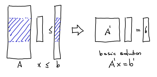
A basic solution can be represented by picking rows of the matrix and making them tight. So, if we have a general LP, we pick some submatrix of which is and the basic solution is just . The lines of matrix can be of three types: they can be , which are corresponding to , that correspond to or corresponding to . There are vectors in total. The size of the support is smaller or equal the number of rows of the form in the basic solution. Therefore the idea to bound the size of the support is to prove that “all basic solutions can be represented by a small number of rows in the form . And this is done using the following:

Lemma 3 Assuming , for any basic solution , there is and a family of sets such that:

1. The restrictions correspondent to and are tight for
2. is an independent set
3. 
4. is a laminar family

The first 3 items are straightfoward properties of basic solutions. The fourth one, means that for two sets , one of three things happen: , or . Now, we based on the previous lemma and in the following result that can be easily proved by induction, we will prove Lemma 1.

Lemma 4 If is a laminar family over the set where each set contains at least elements, then .

Now, the proof of Lemma 1 is easy. Let’s do it and then we come back to prove Lemma 3. Simply see that what contradicts .

Uncrossing argument

And now we arrive in the technical heart of the proof, which is proving Lemma 3. This says that given any basic solution, given any feasible solution, we can write it as a “structured” basic solution. We start with any basic feasible solution. This already satifies (1)-(3), then we need to change that solution to satisfy condition (4) as well. We need to get rid crossing elements, i.e., in the form:

We do that by the means of the:

Lemma 5 (Uncrossing Lemma) If and are intersecting and tight (tight in the sense that their respective constraint is tight), then and are also tight and:

Which corresponds to that picture:

Proof: First, we note that is a supermodular function, i.e.:

We can see that by case analysis. Every edge appearing in the left side appears in the right side with at least the same multiplicity. Notice also that it holds with strict inequality iff there are edges from to . Now, we have:

where the first relation is trivial, the second is by feasibility, the third is by supermodularity and the lastone is by tightness. So, all hold with equality and therefore and are tight. We also proved that:

so there can be no edge from to in and therefore, thinking just of edges in we have:

Uncrossing arguments are found everywhere in combinatorics. Now, we show how the Uncrossing Lemma can be used to prove Lemma 1:

Proof: Let be any basic solution. It can be represented by a pair where and is a family of sets. We will show that the same basic solution can be represented by where is a laminar family and has the same size of .

Let be all sets that are tight under and a maximal laminar family of tights sets in , such that are independent. I claim that .

In fact, suppose , then there are sets of we could add to without violating independence – the problem is that those sets would cross some set. Pick such intersecting fewer possible sets in . The set intersects some . Since both are tight we can use the Uncrossing Lemma and we get:

since , we can’t have simultaneously and in . Let’s consider two cases:

1. , then is in and intersects fewer sets of than , since all sets that intersect in must intersect as well (since no set can cross ).
2. , then is in and intersects fewer sets of than , since all sets that intersect in must intersect .

In either case we have a contradiction, so we proved that . So we can generate all the space of tight sets with a laminar family.

And this finishes the proof. Let’s go over all that we’ve done: we started with an LP and we wanted to prove that the support of each solution was not too large. We wanted that because we wanted to prove that there was one node with degree one in the support or a node in with small () degree. To prove that the degree of the support is small, we show that any basic solution has a representation in terms of a laminar family. Then we use the fact that laminar families can’t be very large families of sets. For that, we use the celebrated Uncrossing Lemma.

Note: Most of this is based on my notes on David Williamson’s Approximation Algorithms class. I spent some time thinking about this algorithm and therefore I decided o post it here.