Big Red Bits

Three interesting puzzles

September 29th, 2011 renatoppl No comments

Here are three puzzles I got from 3 different people recently. The first I got from Charles, who got it from a problem set of the Brazilian Programming Competition.

Puzzle #1: Given $n$ and a vector of in-degrees and out-degrees $\text{in}_i$ and $\text{out}_i$ for $i=1..n$ , find if there is a simple directed graph on $n$ nodes with those in and out-degrees in time $O(n \log n)$ . By a simple directed graph, I mean at most one edge between each pair $(i,j)$ , allowing self loops $(i,i)$ .

Solving this problem in time $O(n^3)$ is easy using a max-flow computation – simply consider a bipartite graph with and edge $(i,j)$ between each pair with capacity $1$ . Add a source and connect to each node in the left size with capacity $\text{in}_i$ and add also a sink in the natural way, compute max-flow and check if it is $\sum_i \text{in}_i$ . But it turns out we can do it in a lot more efficient way. The solution I thought works in time $O(n \log n)$ but maybe there is a linear solution out there. If you know of one, I am curious.

The second puzzle was given to me by Hyung-Chan An:

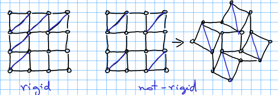
Puzzle #2: There is grid of size $n \times m$ formed by rigid bars. Some cells of the grid have a rigid bar in the diagonal, making that whole square rigid. The question is to decide, given a grid and the location of the diagonal bars if the entire structure is rigid or not. By rigid I mean, being able to be deformed.

We thought right away in a linear algebraic formulation: look at each node and create a variable for each of the 4 angles around it. Now, write linear equations saying that some variables sum to 360, since they are around one node. Equations saying that some variable must be 90 (because it is in a rigid cell). Now, for the variables internal to each square, write that opposite angles must be equal (since all the edges are of equal length) and then you have a linear system of type $Ax = b$ where $x$ are the variables (angles). Now, we need to check if this system admits more then one solution. We know a trivial solution to it, which is all variable is 90. So, we just need to check if the matrix $A$ has full rank.

It turns out this problem has a much more beautiful and elegant solution and it is totally combinatorial – it is based on verifying that a certain bipartite graph is connected. You can read more about this solution in Bracing rectangular frameworks. I by (Bolker and Crapo 1979). A cute idea is to use the the following more general linear system (which works for rigidity in any number of dimensions). Consider a rigid bar from point $p_a \in \mathbb{R}^n$ to point $p_b \in \mathbb{R}^n$ . If the structure is not rigid, then there is a movement it can make: let $v_a$ and $v_b$ be the instantaneous velocities of points $a$ and $b$ . If $p_a(t), p_b(t)$ are the movements of points $a,b$ , then it must hold that: $\Vert p_a(t) - p_b(t) \Vert = \Vert p_a(0) - p_b(0) \Vert$ , so taking derivatives we have:

$(p_a(0) - p_b(0)) \cdot (v_a - v_b) = 0$

This is a linear system in the velocities. Now, our job is to check if there are non zero velocities, which again is to check that the matrix of the linear system is or is not full-rank. Â An interesting thing is that if we look at this question for the grid above, this matrix will be the matrix of a combinatorial problem! So we can simply check if it has full rank by solving the combinatorial problem. Look at the paper for more details.

The third puzzle I found in the amazing website called The Puzzle Toad, which is CMU’s puzzle website:

Puzzle #3: There is a game played between Arthur and Merlin. There is a table with $n$ lamps disposed in a circle, initially some are on and some are off. In each timestep, Arthur writes down the position of the lamps that are off. Then Merlin (in an adversarial way) rotates the table. The Arthur’s servant goes and flips (on –> off, off –> on) the lamps whose position Arthur wrote down (notice now he won’t be flipping the correct lamps, since Merlin rotated the table. if Arthur wrote lamp 1 and Merlin rotated the table by 3 positions, the servant will actually be flipping lamp 4. The question is: given $n$ and an initial position of the table, is there a strategy for Merlin Â such that Arthur never manages to turn all the lamps on.

See here for a better description and a link to the solution. For $n = 2^k$ no matter what Merlin does, Arthur always manages to turn on all the lamps eventually, where eventually means in $O(n^2)$ time. The solution is a very pretty (and simple) algebraic argument. I found this problem really nice.

Categories: puzzles, theory Tags: algorithms, puzzles

Bayesian updates and the Lake Wobegon effect

September 25th, 2011 renatoppl No comments

We seem to have a good mathematical understanding of Bayesian updates, but somehow a very poor understanding of its practical implications. There are many situations in practice that we easily perceive as irrational, one of the most famous is the so calledÂ Lake Wobegon effect, named after theÂ fictional town in Minnesota, where “all the women are strong, all the men are good looking, and all the children are above average”. It is described as a cognitive bias where individuals tend to overestimate their own capabilities. In fact, when drivers are asked to rate their own skilled compared to the average in three groups: low-skilled, medium-skilled and high-skilled, most rate themselves above the average.

In fact, the behavioral economics literate is full of examples like this where the observed data is far from what you would expect to observe if all agents were rational – and those are normally attributed to cognitive biases. I was always a bitÂ suspicious of such arguments: it was never clear if agents were simply not being rational or whether their true objective wasn’t being captured by the model. I always thought the second was a lot more likely.

One of the main problems of the irrationality argument is that they ignore the fact that agents live in a world where its states are not completely observed. InÂ a beautiful paper in Econometrica called “Apparent Overconfidence“, Benoit and Dubra argue that:

“But the simple truism thatÂ most people cannot be better than the median does not imply that most people cannot rationally rate themselves above the median.”

The authors show that it is possible to reverse engineer a signaling scheme such that the data is mostly consistent with the observation. Let me try to give a simple example they give in the introduction: consider that each driver has one of three types of skill: low, medium or high: $\{L,M,H\}$ and $\mathbb{P}(L) = \mathbb{P}(M) = \mathbb{P}(H) = \frac{1}{3}$ . However, they can’t observe this. They can only observe some sample of their driving. Let’s say for simplicity that they can observe a signal $A$ that says if they caused an accident or not. Assume also that the larger that skill of a driver, the higher it is his probability of causing an accident, say:

$\mathbb{P}(A \vert L) = \frac{47}{80}, \mathbb{P}(A \vert L) = \frac{9}{16}, \mathbb{P}(A \vert L) = \frac{1}{20}$

Before observing $A$ each driver things of himself as having probability $\frac{1}{3}$ of having each type of skill. Now, after observing $A$ , they update their belief according to Bayes rule, i.e.,

$\mathbb{P}(s \vert A) = \frac{ \mathbb{P}(A \vert s) \mathbb{P}(s) }{ \sum_{s'} \mathbb{P}(A \vert s') \mathbb{P}(s') }$

doing the calculations, we have that $\mathbb{P}(A) = \frac{2}{5}$ and for the $\frac{3}{5}$ of the drivers that didn’t suffer an accident, they’ll evaluateÂ $\mathbb{P}(L \vert \neg A) = \frac{11}{48}$ , $\mathbb{P}(M \vert \neg A) = \frac{35}{144}$ , $\mathbb{P}(H \vert \neg A) = \frac{19}{36}$ , so:

$\mathbb{P}(H \vert \neg A) > \mathbb{P}(L \cup M \vert \neg A)$

and therefore will report high-skill. Notice this is totally consistent with rational Bayesian-updaters. The main question in the paper is: “when it is possible to reverse engineer a signaling scheme ?”. More formally, let $\Theta$ be a set of types of users and let $\theta \sim H \in \Delta(\Theta)$ , i.e., $H$ is a distribution on the types which is common knowledge. Now, if we ask agents to report their type, their report is some $H' \in \Delta(\Theta), H' \neq H$ . Is there a signaling scheme $S$ which can be interpreted as a random variable correlated with $\theta$ such that $H'$ is the distribution rational Bayesian updaters would report based on what they observed from $S$ ? The authors give necessary and sufficient condition on when this is possible given $H,H'$ .

—————————–

A note also related to the Lake Wobegon effect: I started reading a very nice book by Duncan Watts called “Everything Is Obvious: *Once You Know the Answer” about traps of the common-sense. The discussion is different then above, but it also talks about the dangers of applying our usual common sense, which is very useful to our daily life, to scientific results. I highly recommend reading the intro of the book, which is open in Amazon. He gives examples of social phenomena where, once you are told them, you think: “oh yeah, this is obvious”. But then if you were told the exact opposite (in fact, he begins the example by telling you the opposite from the observed in data), you’d also think “yes, yes, this is obvious” and come up with very natural explanations. His point is that common sense is very useful to explaining data observations, specially observations of social data. On the other hand, it is performs very poorly on predicting how the data will look like before actually seeing it.

Categories: theory Tags: economics, probability

MHR, Regular Distributions and Myerson’s Lemma

May 30th, 2011 renatoppl No comments

Monotone Hazard Rate (MHR) distributions and its superclass regular distributions keep appearing in the Mechanism Design literature and this is due to a very good reason: they are the class of distributions for which Myerson’s Optimal Auction is simple and natural. Let’s brief discuss some properties of those distributions. First, two definitions:

Hazard rate of a distribution $f$ : $h(z) = \frac{f(z)}{1-F(z)}$
Myerson virtual value of a distribution $f$ : $\phi(z) = z - \frac{1-F(z)}{f(z)}$

We can interpret the hazard rate in the following way: think of $T \sim f$ as a random variable that indicates the time that a light bulb will take to extinguish. If we are in time $t$ and the light bulb hasn’t extinguished so far, what is the probability it will extinguish in the next $\delta$ time:

$\mathbb{P}[T \leq t+\delta \vert T > t] \approx \frac{f(t) \delta}{1-F(t)}$

We say that a distribution is monotone hazard rate, if $h(z)$ is non-decreasing. This is very natural for light bulbs, for example. Many of the distributions that we are used to are MHR, for example, uniform, exponential and normal. The way that I like to think about MHR distributions is the following: if some distribution has hazard rate $h(z)$ , then it means that $F'(z) = (1-F(z)) h(z)$ . If we define $G(z) = 1-F(z)$ , then $(log G(z))' = \frac{G'(z)}{G(z)} = -h(z)$ , so:

$F(z) = 1-\text{exp}(-\int_0^z h(u) du)$

From this characterization, it is simple to see that the extremal distributions for this class, i.e. the distributions that are in the edge of being MHR and non-MHR are constant hazard rate, which correspond to the exponential distribution $F(z) = 1-e^{-\lambda z}$ for $z \in [0,\infty)$ . They way I like to think about those distributions is that whenever you are able to prove something about the exponential distribution, then you can prove a similar statement about MHR distributions. Consider those three examples:

Example 1: $\mathbb{P}[\phi(z) \geq 0] \geq \frac{1}{e}$ for MHR distributions. This fact is straightforward for the exponential distribution. For the exponential distribution $\phi(z) = z-\lambda^{-1}$ and therefore

$\mathbb{P}[\phi(z) \geq 0] \geq \mathbb{P}[z > \lambda^{-1}] = 1-F(\lambda^{-1}) = e^{-1}$

but the proof for MHR is equally simple: Let $r = \inf \{z; \phi(z) \geq 0\}$ , therefore $r h(r) \leq 1$ .
$P\{ \phi(v) \geq 0\} = P\{ v \geq r \} = 1 - F(r) = e^{-\int_0^r h(u) du} \geq e^{-r h(r)} \geq e^{-1}$

Example 2: Given $z_1, z_2 \sim f$ iid where $f$ is MHR and $v_1 = \max \{z_1, z_2\}$ and $v_2 = \min \{z_1, z_2\}$ , then $\mathbb{E}[v_2] \geq \frac{1}{3} \mathbb{E}[v_1]$ . The proof for the exponential distribution is trivial, and in fact, this is tight for the exponential, the trick is to use the convexity of $z \mapsto \int_0^z h(u) du$ . We use that $\int_0^{2z} h \geq 2 \int_0^z h$ in the following way:

$\mathbb{E} [v_2] = \int_0^\infty (1 - F(z))^2 dz = \int_0^\infty e^{-2 \int_0^z h} dz$

$\geq \int_0^\infty e^{-\int_0^{2z} h} dz= \frac{1}{2} \int_0^\infty 1 - F(z) dz = \frac{1}{2} \mathbb{E} [z]$

Since $\mathbb{E} [v_1 + v_2] = \mathbb{E} [z_1 + z_2] = 2 \mathbb{E} [z]$ , we have that $\mathbb{E}[v_1] = 2 \mathbb{E}[z] - \mathbb{E}[v_2] \leq \frac{3}{2} \mathbb{E}[z]$ . This way, we get: $\mathbb{E}[v_2] \geq \frac{1}{2}\mathbb{E}[z] \geq \frac{1}{2} \cdot \frac{2}{3} \mathbb{E}[v_1] = \frac{1}{3} \mathbb{E}[v_1]$

Example 3: For MHR distributions, there is a simple lemma that relates the virtual value and the real value and this lemma is quite useful in various settings: let $r = \inf \{z; \phi(z) > 0 \}$ , then for $z \geq r$ , $\phi(z) \geq z - r$ . Again, this is tight for exponential distribution. The proof is quite trivial:

$x - \phi(x) = \frac{1-F(x)}{f(x)} \leq \frac{1-F(r)}{f(r)} = r$

Now, MHR distributions are a subclass of regular distributions, which are the distributions for which Myerson’s virtual value $\phi(z)$ is a monotone function. I usually find harder to think about regular distributions than to think about MHR (in fact, I don’t know so many examples that are regular, but not MHR. Here is one, though, called the equal-revenue-distribution. Consider $z \in [1, \infty)$ distributed according to $f(z) = 1/z^2$ . The cumulative distribution is given by $F(z) = 1-1/z$ . The interesting thing of this distribution is that posted prices get the same revenue regardless of the price. For example, if we post any price $r \in [1,\infty)$ , then a customer with valuations $z \sim f$ buys the item if $z > r$ by price $r$ , gettingÂ revenue is $r (1-F(r)) = 1$ . This can be expressed by the fact that $\phi(z) = 0$ . I was a bit puzzled by this fact, because of Myerson’s Lemma:

Myerson Lemma: If a mechanism sells to some player that has valuation $v \sim f$ with probability $x(v)$ when he has value $v$ , then the revenue is $\mathbb{E} [x(v) \phi(v)]$ .

And it seemed that the auctioneers was doomed to get zero revenue, since $\phi(z) = 0$ . For example, suppose we fix some price $r$ and we sell the item if $v \geq r$ by price $r$ . Then it seems that Myerson’s Lemma should go through by a derivation like that (for this special case, although the general proof is quite similar):

$\mathbb{E} [x(v) \phi(v)] = \int_r^\infty \phi(z) f(z) dz = \int_r^\infty z f(z) - (1-F(z)) dz =$

$= \int_r^\infty [ z f(z) - \int_z^\infty f(u) du ] dz = \int_r^\infty z f(z) dz - \int_r^\infty \int_r^u f(u) dz du$

$= r (1-F(r))$

but those don’t seem to match, since one side is zero and the other is 1. The mistake we did above is classic, which is to calculate $\infty - \infty$ . We wrote:

$\mathbb{E}[\phi(v)] = \int_r^\infty z f(z) dz - \int_r^\infty 1-F(z) dz$

but both are infinity! This made me realize that Myerson’s Lemma needs the condition that $\mathbb{E}[z] < \infty$ , which is quite a natural a distribution over valuations of a good. So, one of the bugs of the the equal-revenue-distribution is that $\mathbb{E}[z] = \infty$ . A family that is close to this, but doesn’t suffer this bug is: $f(z) = \frac{\alpha-1}{z^\alpha}$ for $z \in [1,\infty)$ , then $F(z) = 1 - z^{1-\alpha}$ . For $\alpha > 2$ we have $\mathbb{E}[v] < \infty$ , then we get $\phi(z) = \frac{\alpha-2}{\alpha-1} z$ .