Archive

Posts Tagged ‘combinatorics’

Bounded Degree Spanning Tree and an Uncrossing Lemma

November 17th, 2009 No comments

I’ve been reading about the Bounded Degree Spanning Tree problem and I thought of writing some of what I am learning here. It illustrates a beautiful techique called Iterated Rounding and uses the combinatorial idea of uncrossing. I’ll try to give a high-level idea of the argument and give references on the details. The first result of this kind was given by Goemans (although there were previous results with weaker guarantees) by Goemans in Minimum Bounded Degree Spanning Trees, but the result based on iterated rounding and a subsequent improvement are due to Singh and Lau in a serie of papers. A main reference is Approximating minimum bounded degree spanning trees to within one of optimal.

The problem of bounded degree spanning tree is as follows: consider a graph {G = (V,E)} with edge weights and we for some nodes {W \subseteq V} a degree bound {b_v, v \in W}. We want to find, among the spanning trees for which the degree of {v} is {\leq b_v} the one with minimum cost. It is clearly a hard problem, since taking all weights equal to {1} and {b_v = 2} for all nodes is the Hamiltonian Path problem, which is NP-complete. We will get a different kind of approximation. Let OPT be the optimal solution: we will show an algorithm that gives a spanning tree of cost {\leq OPT} such that each node {v} has degree {\leq b_v + 2} (this can be improved to {b_v + 1} with a more sofisticated algorithm, also based on Iterated Rounding).

As always, the first step to design an approximation algorithm is to relax it to an LP. We consider the following LP:

\displaystyle \left. \begin{aligned} & \min \sum_{e\in E} c_e x_e \text{ s.t. } \\ & \qquad \left. \begin{aligned} & \sum_{e \in E} x_e = \vert V \vert - 1 \\ & \sum_{e \in E(S)} x_e \leq \vert S \vert - 1 & \forall S \subseteq V, \vert S \vert \geq 2 \\ & \sum_{e \in \delta(v)} x_e \leq b_v & \forall v \in W\\ & x_e \geq 0 & \forall e \in E \end{aligned} \right. \end{aligned} \right.

The first constraint expresses that in a spanning tree, there are at most {\vert V \vert - 1} edges, the second prevent the formation of cycles and the third guarantees the degree bounds. For {W = \emptyset} we have the standard Minimal Spanning Tree problem and for this problem the polytope is integral. With the degree bounds, we lose this nice property. We can solve this LP using the Ellipsoid Method. The separation oracle for the {\sum_{e \in E(S)} x_e \leq \vert S \vert - 1} is done by a flow computation.

Iterated Rounding

Now, let’s go ahead and solve the LP. It would be great if we had an integral solution: we would be done. It is unfortunately not the case, but we can still hope it is almost integral in some sense: for example, some edges are integral and we can take them to the final solution and recurse the algorithm on a smaller graph. This is not far from truth and that’s the main idea of the iterated rounding. We will show that the support of the optimal solution {E(x) = \{e \in E; x_e > 0\}} has some nice structure. Consider the following lemma:

Lemma 1 For any basic solution {x} of the LP, either there is {v} with just one incident edge in the support {E(x)} or there is one {v \in W} such that that at most {3} edges are incident to it.

If we can prove this lemma, we can solve the problem in the following way: we begin with an empty tree: then we solve the LP and look at the support {E(x)}. There are two possibilities according to the lemma:

  • If there is one node {v} with just one edge {e = (u,v)} incident to it in the support, we add it to the tree, remove {v} from {V}, decrease {b_u}, make {E = E(x)} (the trick is to remove in each iteration edges from {E} that are not in the support. Clearly, removing those edges doesn’t hurt the objective value) and run the algorithm again. Notice that the LP called in the recursion has value less or equal then the actual LP {- c_e}. So if by induction we get a spanning tree respecting the new degree bounds plus two and value less or equal than the new LP value, we can just add {e} and we have a solution with value less or equal than the one of the original LP respecting the degree bounds plus two.
  • Otherwise, there is one node {v \in W} that has degree {3} in the support. So, we just remove that degree bound on that vertex (i.e. remove {v} from {W}), make {E = E(x)} (again,eliminate the edges not in the support) and run the algorithm again. Clearly, if one node is still in {W}, it has {b_v \geq 1}, since there are only three edges in the support, there will be for the rest of the computation, just three edges incident to it, so there will be at most three edges more incident to it. So it will exceed its original {b_v} by at most {2}.

The algorithm eventually stops, since in each iteration we have less edges or less nodes in {W} and the solution is as desired. The main effort is therefore to prove the lemma. But before, let’s look at the lemma: it is of the following kind: “any basic solution of the LP has some nice properties, which envolve having a not too big (at least in some point) support”. So, it involves proving that the support is not too large. That is our next task as we are trying to prove the lemma. And we will be done with:

Theorem 2 The algorithm described above produces a spanning tree of cost {\leq Z^*} (the LP values and therefore {\leq OPT})in which each node {v \in W} has degree {\leq b_v + 2}.

Bounding the size of the support

We would like now to prove some result like the Lemma above: that in the solution of the LP we have either one {v} with degree {1} in {E(x)} or we have a node in {W} with degree {\leq 3}. First, we suppose the opposite, that {(V,E(x))} has all the nodes with degree {\geq 2} and all the nodes in {W} have degree {\geq 4}. This implies that we have a large number of edges in the support. From the degrees, we know that:

\displaystyle \vert E(x) \vert \geq \frac{1}{2} \left( 2( \vert V \vert - \vert W \vert ) + 4 \vert W \vert \right) = \vert V \vert + \vert W \vert

We want to prove that the support {\vert E(x) \vert} of the LP can’t be too large. The first question is: how to estimate the size of the support of a basic solution. The constraints look like that:
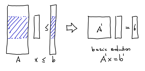
bst_fig1

A basic solution can be represented by picking {\vert E \vert} rows of the matrix and making them tight. So, if we have a general {Ax \leq b} LP, we pick some submatrix {A'} of {A} which is {n \times n} and the basic solution is just {x = A'^{-1} b'}. The lines of matrix {A'} can be of three types: they can be {\chi_S}, which are corresponding to {\sum_{e \in E(S)} x_e \leq \vert S \vert - 1}, {\chi_v} that correspond to {\sum_{e \in \delta(v)} x_e \leq b_v} or {\delta_e} corresponding to {x_e \geq 0}. There are {\vert E \vert} vectors in total. The size of the support {E(x)} is smaller or equal the number of rows of the form {\chi_S, \chi_v} in the basic solution. Therefore the idea to bound the size of the support is to prove that “all basic solutions can be represented by a small number of rows in the form {\chi_S, \chi_v}. And this is done using the following:

Lemma 3 Assuming {E = E(x)}, for any basic solution {x}, there is {Z \subseteq W} and a family {\mathcal{S}} of sets such that:

  1. The restrictions correspondent to {S \in \mathcal{S}} and {v \in Z} are tight for {x}
  2. {\{ \chi_S; S \in \mathcal{S} \} \cup \{ \chi_v; v \in Z \}} is an independent set
  3. {\vert \mathcal{S} \vert + \vert Z \vert = \vert E(x) \vert}
  4. {\mathcal{S}} is a laminar family

The first 3 items are straightfoward properties of basic solutions. The fourth one, means that for two sets {S_1, S_2 \in \mathcal{S}}, one of three things happen: {S_1 \subseteq S_2}, {S_2 \subseteq S_1} or {S_1 \cap S_2 = \emptyset}. Now, we based on the previous lemma and in the following result that can be easily proved by induction, we will prove Lemma 1.

Lemma 4 If {\mathcal{S}} is a laminar family over the set {V} where each set {S \in \mathcal{S}} contains at least {2} elements, then {\vert \mathcal{S} \vert \leq \vert V \vert - 1}.

Now, the proof of Lemma 1 is easy. Let’s do it and then we come back to prove Lemma 3. Simply see that {\vert E(x) \vert = \vert \mathcal{S} \vert + \vert Z \vert \leq \vert V \vert - 1 + \vert W \vert} what contradicts {\vert E(x) \vert \geq \vert V \vert + \vert W \vert}.

Uncrossing argument

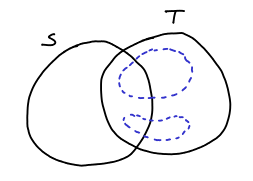
And now we arrive in the technical heart of the proof, which is proving Lemma 3. This says that given any basic solution, given any feasible solution, we can write it as a “structured” basic solution. We start with any basic feasible solution. This already satifies (1)-(3), then we need to change that solution to satisfy condition (4) as well. We need to get rid crossing elements, i.e., {S,T \in \mathcal{S}} in the form:

bst_fig2

We do that by the means of the:

Lemma 5 (Uncrossing Lemma) If {S} and {T} are intersecting and tight (tight in the sense that their respective constraint is tight), then {S \cup T} and {S \cap T} are also tight and:

\displaystyle \chi_{S \cap T} + \chi_{S \cup T} = \chi_S + \chi_T

Which corresponds to that picture:

bst_fig3

Proof: First, we note that {x(E(S))} is a supermodular function, i.e.:

\displaystyle x(E(S)) + x(E(T)) \leq x(E(S \cap T)) + x(E(S \cup T))

We can see that by case analysis. Every edge appearing in the left side appears in the right side with at least the same multiplicity. Notice also that it holds with strict inequality iff there are edges from {S\setminus T} to {T \setminus S}. Now, we have:

\displaystyle \begin{aligned} (\vert S \vert - 1) + (\vert T \vert - 1) & = (\vert S \cap T \vert - 1) + (\vert S \cup T \vert - 1) \geq \\ & \geq x(E(S \cap T)) + x(E(S \cup T)) \geq \\ & \geq x(E(S)) + x(E(T)) = (\vert S \vert - 1) + (\vert T \vert - 1) \end{aligned}

where the first relation is trivial, the second is by feasibility, the third is by supermodularity and the lastone is by tightness. So, all hold with equality and therefore {S \cap T} and {S \cup T} are tight. We also proved that:

\displaystyle x(E(S \cap T)) + x(E(S \cup T)) = x(E(S)) + x(E(T))

so there can be no edge from {S\setminus T} to {T \setminus S} in {E(x)} and therefore, thinking just of edges in {E(x)} we have:

\displaystyle \chi_{S \cap T} + \chi_{S \cup T} = \chi_S + \chi_T

\Box

Uncrossing arguments are found everywhere in combinatorics. Now, we show how the Uncrossing Lemma can be used to prove Lemma 1:

Proof: Let {x} be any basic solution. It can be represented by a pair {(Y, \mathcal{C})} where {Y \subseteq W} and {\mathcal{C}} is a family of sets. We will show that the same basic solution can be represented by {(Y, \mathcal{L})} where {\mathcal{L}} is a laminar family and has the same size of {\mathcal{C}}.

Let {\mathcal{S}} be all sets that are tight under {x} and {\mathcal{L}} a maximal laminar family of tights sets in {\mathcal{S}}, such that {\{\chi_S; S \in \mathcal{L} \} \cup \{\chi_v; v \in Z \}} are independent. I claim that {\vert \mathcal{L} \vert = dim(span(\mathcal{S}))}.

In fact, suppose {\vert \mathcal{L} \vert < dim(span(\mathcal{S}))}, then there are sets of {\mathcal{S}} we could add to {\mathcal{L}} without violating independence – the problem is that those sets would cross some set. Pick such {S \in \mathcal{S}} intersecting fewer possible sets in {\mathcal{L}}. The set {S} intersects some {T \in \mathcal{L}}. Since both are tight we can use the Uncrossing Lemma and we get:

\displaystyle \chi_{S \cap T} + \chi_{S \cup T} = \chi_S + \chi_T

since {\chi_S \notin span(\mathcal{L})}, we can’t have simultaneously {\chi_{S \cap T}} and {\chi_{S \cup T}} in {span(\mathcal{L})}. Let’s consider two cases:

  1. {\chi_{S \cap T} \notin span(\mathcal{L})}, then {S \cap T \in span(\mathcal{S})} is in {span(\mathcal{S}) \setminus span(\mathcal{L})} and intersects fewer sets of {\mathcal{L}} than {S}, since all sets that intersect {S \cap T} in {\mathcal{L}} must intersect {S} as well (since no set can cross {T}).bst_fig4
  2. {\chi_{S \cup T} \notin span(\mathcal{L})}, then {S \cup T \in span(\mathcal{S})} is in {span(\mathcal{S}) \setminus span(\mathcal{L})} and intersects fewer sets of {\mathcal{L}} than {S}, since all sets that intersect {S \cup T} in {\mathcal{L}} must intersect {S}.

In either case we have a contradiction, so we proved that {\vert \mathcal{L} \vert = dim(span(\mathcal{S}))}. So we can generate all the space of tight sets with a laminar family. \Box

And this finishes the proof. Let’s go over all that we’ve done: we started with an LP and we wanted to prove that the support of each solution was not too large. We wanted that because we wanted to prove that there was one node with degree one in the support or a node in {W} with small ({\leq 3}) degree. To prove that the degree of the support is small, we show that any basic solution has a representation in terms of a laminar family. Then we use the fact that laminar families can’t be very large families of sets. For that, we use the celebrated Uncrossing Lemma.

Note: Most of this is based on my notes on David Williamson’s Approximation Algorithms class. I spent some time thinking about this algorithm and therefore I decided o post it here.

Random Spanning Trees

November 3rd, 2009 No comments

BigRedBits is again pleased to have Igor Gorodezky as a guest blogger directly from UCLA. I leave you with his excelent post on the Wilson’s algorithm.

——————————————

Igor again, with another mathematical dispatch from UCLA, where I’m spending the semester eating and breathing combinatorics as part of the 2009 program on combinatorics and its applications at IPAM. In the course of some reading related to a problem with which I’ve been occupying myself, I ran across a neat algorithmic result – Wilson’s algorithm for uniformly generating spanning trees of a graph. With Renato’s kind permission, let me once again make myself at home here at Big Red Bits and tell you all about this little gem.

The problem is straightforward, and I’ve essentially already stated it: given an undirected, connected graph {G}, we want an algorithm that outputs uniformly random spanning trees of {G}. In the early ’90s, Aldous and Broder independently discovered an algorithm for accomplishing this task. This algorithm generates a tree {T} by, roughly speaking, performing a random walk on {G} and adding the edge {(u,v)} to {T} every time that the walk steps from {u} to {v} and {v} is a vertex that has not been seen before.

Wilson’s algorithm (D. B. Wilson, “Generating random spanning trees more quickly than the cover time,” STOC ’96) takes a slightly different approach. Let us fix a root vertex {r}. Wilson’s algorithm can be stated as a loop-erased random walk on {G} as follows.

Algorithm 1 (Loop-erased random walk) Maintain a tree {T}, initialized to consist of {r} alone. While there remains a vertex {v} not in {T}: perform a random walk starting at {v}, erasing loops as they are created, until the walk encounters a vertex in {T}, then add to {T} the cycle-erased simple path from {v} to {T}.

We observe that the algorithm halts with probability 1 (its expected running time is actually polynomial, but let’s not concern ourselves with these issues here), and outputs a random directed spanning tree oriented towards {r}. It is a minor miracle that this tree is in fact sampled uniformly from the set of all such trees. Let us note that this offers a solution to the original problem, as sampling {r} randomly and then running the algorithm will produce a uniformly generated spanning tree of {G}.

It remains, then, to prove that the algorithm produces uniform spanning trees rooted at {r} (by which we mean directed spanning trees oriented towards {r}). To this we dedicate the remainder of this post.

1. A “different” algorithm

Wilson’s proof is delightfully sneaky: we begin by stating and analyzing a seemingly different algorithm, the cycle-popping algorithm. We will prove that this algorithm has the desired properties, and then argue that it is equivalent to the loop-erased random walk (henceforth LERW).

The cycle-popping algorithm works as follows. Given {G} and {r}, associate with each non-root vertex {v} an infinite stack of neighbors. More formally, to each {v \neq r} we associate

\displaystyle  \mathcal S_v = [u_{0}, u_{1}, \dots ]

where each {u_{i}} is uniformly (and independently) sampled from the set of neighbors of {v}. Note that each stack is not a random walk, just a list of neighbors. We refer to the left-most element above as the top of {\mathcal S_v}, and by popping the stack {\mathcal S_v} we mean removing this top vertex from {\mathcal S_v}.

Define the stack graph {G_{\mathcal S}} to be the directed graph on {V} that has an edge from {v} to {u} if {u} is at the top of the stack {\mathcal S_v}. Clearly, if {G} has {n} vertices then {G_{\mathcal S}} is an oriented subgraph of {G} with {n-1} edges. The following lemma follows immediately.

Lemma 1 Either {G_{\mathcal S}} is a directed spanning tree oriented towards {r} or it contains a directed cycle.

If there is a directed cycle {C} in {G_{\mathcal S}} we may pop it by popping {\mathcal S_v} for every {v \in C}. This eliminates {C}, but of course might create other directed cycles. Without resolving this tension quite yet, let us go ahead and formally state the cycle-popping algorithm.

Algorithm 2 (Cycle-popping algorithm) Create a stack {\mathcal S_v} for every {v \neq r}. While {G_{\mathcal S}} contains any directed cycles, pop a cycle from the stacks. If this process ever terminates, output {G_{\mathcal S}}.

Note that by the lemma, if the algorithm ever terminates then its output is a spanning tree rooted at {r}. We claim that the algorithm terminates with probability 1, and moreover generates spanning trees rooted at {r} uniformly.

To this end, some more definitions: let us say that given a stack {\mathcal S_v}, the vertex {u_i} is at level {i}. The level of a vertex in a stack is static, and is defined when the stack is created. That is, the level of {u_i} does not change even if {u_i} advances to the top of the stack as a result of the stack getting popped.

We regard the sequence of stack graphs produced by the algorithm as leveled stack graphs: each non-root vertex {v} is assigned the level of its stack. Observe that the level of {v} in {G_{\mathcal S}} is the number of times that {\mathcal S_v} has been popped. In the same way, we regard cycles encountered by the algorithm as leveled cycles, and we can regard the tree produced by the algorithm (if indeed one is produced) as a leveled tree.

The analysis of the algorithm relies on the following key lemma (Theorem 4 in Wilson’s paper), which tells us that the order in which the algorithm pops cycles is irrelevant.

Lemma 2 For a given set of stacks, either the cycle-popping algorithm never terminates, or there exists a unique leveled spanning tree {T} rooted at {r} such that the algorithm outputs {T} irrespective of the order in which cycles are popped.

Proof: Fix a set of stacks {\{ \mathcal S_v \}_{v \neq r}}. Consider a leveled cycle {C} that is pop-able, i.e.~there exist leveled cycles {C_1, C_2, \dots, C_k=C} that can be popped in sequence. We claim that if the algorithm pops any cycle not equal to {C}, then there still must exist a series of cycles that ends in {C} and that can be popped in sequence. In other words, if {C} is pop-able then it remains pop-able, no matter which cycles are popped, until {C} itself is actually popped.

Let {C'} be a cycle popped by the algorithm. If {C'=C_1} then the claim is clearly true. Also, if {C'} shares no vertices with {C_1, \dots, C_k}, then the claim is true again. So assume otherwise, and let {C_i} be the first in the series {C_1, \dots, C_k} to share a vertex with {C'}. Let us show that {C'=C_i} by contradiction.

If {C_i \neq C'}, then {C_i} and {C'} must share a vertex {w} that has different successors in {C'} and {C_i}. But by definition of {C_i}, none of the {C_1, \dots, C_{i-1}} contain {w}, and this implies that {w} has the same level in {C'} and {C_i}. Therefore its successor in both cycles is the same, a contradiction. This proves {C_i=C'}.

Moreover, the argument above proves that {C_i} and {C'} are equal as leveled cycles (i.e.~every vertex has the same level in both cycles). Hence

\displaystyle  C'=C_i, C_1, C_2, \dots, C_{i-1}, C_{i+1}, \dots, C_k=C

is a series of cycles that can be popped in sequence, which proves the original claim about {C}.

We conclude that given a set of stacks, either there is an infinite number of pop-able cycles, in which case there will always be an infinite number and the algorithm will never terminate, or there is a finite number of such cycles. In the latter case, every one of these cycles is eventually popped, and the algorithm produces a spanning tree {T} rooted at {r}. The level of each non-root vertex in {T} is given by (one plus) the number of popped cycles that contained {v}. \Box

Wilson summarizes the cycle-popping algorithm thusly: “[T]he stacks uniquely define a tree together with a partially ordered set of cycles layered on top of it. The algorithm peels off these cycles to find the tree.”

Theorem 3 The cycle-popping algorithm terminates with probability 1, and the tree that it outputs is a uniformly sampled spanning tree rooted at {r}.

Proof: The first claim is easy: {G} has a spanning tree, therefore it has a directed spanning tree oriented towards {r}. The stacks generated in the first step of the algorithm will contain such a tree, and hence the algorithm will terminate, with probability 1.

Now, consider a spanning tree {T} rooted at {r}. We’ll abuse notation and let {T} be the event that {T} is produced by the algorithm. Similarly, given a collection of leveled cycles {\mathcal C}, we will write {\mathcal C} for the event that {\mathcal C} is the set of leveled cycles popped by the algorithm before it terminates. Finally, let {\mathcal C \wedge T} be the event that the algorithm popped the leveled cycles in {\mathcal C} and terminated, with the resulting leveled tree being equal to {T}.

By the independence of the stack entries, we have {\Pr[\mathcal C \wedge T] = \Pr[\mathcal C] \cdot p}, where {p} is the probability that the algorithm’s output is a leveled version of {T}, a quantity which a moment’s reflection will reveal is independent of {T}. Now,

\displaystyle  \Pr[T] = \sum_{\mathcal C} \Pr[\mathcal C \wedge T] = p \sum_{\mathcal C} \Pr[\mathcal C]

which, as desired, is independent of {T}. \Box

2. Conclusion

We have shown that the cycle-popping algorithm generates spanning trees rooted at {r} uniformly. It remains to observe that the LERW algorithm is nothing more than an implementation of the cycle-popping algorithm! Instead of initially generating the (infinitely long) stacks and then looking for cycles to pop, the LERW generates stack elements as necessary via random walk (computer scientists might recognize this as the Principle of Deferred Decisions). If the LERW encounters a loop, then it has found a cycle in the stack graph {G_{\mathcal S}} induced by the stacks that the LERW has been generating. Erasing the loop is equivalent to popping this cycle. We conclude that the LERW algorithm generates spanning trees rooted at {r} uniformly.

Categories: theory Tags: , ,

Using expanders to prove sum-product inequalities in finite fields

September 23rd, 2009 No comments

I am happy to have the first guest post of BigRedBits written by Igor Gorodezky about an elegant and exciting result in combinatorics.

————————-

I’m fortunate enough to be spending this semester in beautiful Los Angeles as a core participant in the 2009 long program on combinatorics at IPAM (an NSF-funded math institute on UCLA’s campus). We’ve recently wrapped up the first part of the program, which consisted of tutorial lectures on various topics in combinatorics. There was an abundance of gorgeous mathematics, and with Renato’s kind permission I’d like to hijack his blog and write about what to me was one of the most memorable lectures.

This was a lecture by Jozsef Solymosi of the University of British Columbia describing some of his recent work on the sum-product problem in finite fields. In particular, he outlined a spectral-graph-theoretic proof of a recent sum-product inequality due to Garaev. Solymosi’s proof is an extremely clever and elegant application of spectral graph theory to a classical problem in combinatorial number theory, and so I thought I’d present it here. Before stating the result and giving Solymosi’s proof, let us begin with a very brief introduction to the sum-product problem.

1. Introduction

Given a finite set of real numbers {A}, define the sum set

\displaystyle  A+A = \{a+b \mid a,b \in A\}

and the product set

\displaystyle  A \cdot A = \{ab \mid a,b \in A\}.

Both the sum set and the product set clearly must have cardinality between {|A|} and {|A|^2}. Observe that if {A} is an arithmetic progression then {|A+A| \approx 2|A|} while {|A \cdot A| \approx |A|^2}, while if {A} is a geometric progression then {|A \cdot A| \approx 2|A|} while {|A + A| \approx |A|^2}. Intuition suggests that keeping {|A+A|} small by giving {A} lots of additive structure inevitably blows up {|A \cdot A|}, while keep {|A \cdot A|} small by giving {A} lots of multiplicative structure in turn blows up {|A+A|}. For an arbitrary {A}, one would expect at least one of these sets, if not both, to be fairly large.

Estimating the maximum of {|A+A|} and {|A \cdot A|} is the sum-product problem. It was posed in a paper by Erdos and Szemeredi, who proved the existence of a small constant {c} such that

\displaystyle  \max\{ |A+A|, |A \cdot A| \} = \Omega\left( |A|^{1+c} \right)

for any finite {A}. They conjecture that we actually have

\displaystyle  \max\{ |A+A|, |A \cdot A| \} = \Omega\left( |A|^{2-\delta} \right)

for any {\delta > 0} and sufficiently large {|A|}. In other words, the value of {c} in their bound can be made arbitrarily close to 1.

Much ink has been spilled in attempts to push up the value of {c}. At present, the best sum-product bound is due to Solymosi and gives {c \approx 3/11}. As an aside, I want to mention an extremely simple and elegant probabilistic proof of Elekes that gives {c=1/4}; it is detailed in Alon and Spencer’s classic text The Probabilistic Method, and is an absolute gem (look in the chapter on crossing numbers of graphs).

2. The finite field variant

Solymosi’s IPAM lecture was not, however, on this original sum-product problem, but rather on its natural finite field analogue: if {A} is a subset of {\mathbb F_p}, the finite field of prime order {p}, what can we say about the maximum of {|A+A|} and {|A \cdot A|}? Observe that it is important to consider fields whose order is prime and not the power of a prime, for in the latter case we could take {A} to be a subring and end up with the degenerate case {|A|=|A+A|=|A \cdot A|}.

Bourgain, Katz and Tao got the party started in 2004 by proving the following sum-product bound.

Theorem 1 For all {\epsilon > 0} there exists {\delta > 0} such that if {A \subseteq \mathbb F_p } with {p^{\epsilon} < |A| < p^{1+\epsilon}} then

\displaystyle  \max\{ |A+A|, |A \cdot A| \} = \Omega\left( |A|^{1+\delta} \right).

We note that the implied constant also depends on {\epsilon}. The best known bound is the following, due to Garaev (2007).

Theorem 2 If {A \subseteq \mathbb F_p} then

\displaystyle  \max\{ |A+A|, |A \cdot A| \} = \Omega\left( \min\left\{ |A|^{1/2}p^{1/2},|A|^2p^{-1/2} \right\} \right).

To illustrate the theorem, observe that if {|A| \approx p^{2/3}} then {\max\{ |A+A|, |A \cdot A| \} = \Omega( |A|^{5/4})}. It is this theorem that Solymosi proves using spectral graph theory (Garaev’s original proof went by way of Fourier analysis and the estimation of exponential sums).

3. Solymosi’s proof

In this section we give Solymosi’s proof of Theorem 2 (we will assume familiarity with basic facts about eigenvalues and eigenvectors of adjacency matrices). Let us first establish some notation. Consider a {d}-regular graph {G} and let the eigenvalues of its adjacency matrix be

\displaystyle  d=\lambda_1 \geq \lambda_2 \geq \dots \geq \lambda_n.

As usual, we define

\displaystyle  \lambda(G) = \max\{ \lambda_2,|\lambda_n|\}.

Recall that if {G} is connected and non-bipartite then {\lambda(G)} is strictly smaller than {d}, and such a graph is an expander if {d-\lambda(G)} is bounded below by some constant.

We will make use of a fundamental result in spectral graph theory: the expander mixing lemma.

Lemma 3 Let {G} be a {d}-regular graph with {n} vertices. For all {S,T \subseteq V(G)} we have

\displaystyle  \left| e(S,T) - \frac{d}{n}|S||T| \right| \leq \lambda(G) \sqrt{|S||T|}

where {e(S,T)} is the number of edges with one endpoint in {S} and the other in {T}.

The proof of the lemma is straightforward; we omit it because of space considerations, but it can be found in the survey on expanders by Linial, Hoory, and Wigderson.

Now, back to Theorem 2: we have a finite field {\mathbb F_p} and a subset {A}. Solymosi proves the desired lower bound on {\max\{ |A+A|, |A \cdot A| \}} by constructing a sum-product graph {G_{SP}} over {\mathbb F_p} and using its spectral properties to reason about {|A+A|} and {|A \cdot A|}. So without further ado, let’s define {G_{SP}}.

The vertex set of {G_{SP}} is {\left( \mathbb F_p \setminus \{0\} \right) \times \mathbb F_p}, and two vertices {(a,b),(c,d)} have an edge between them if {ac=b+d}. It is easy to see that {G_{SP}} has {p(p-1)} vertices and is {(p-1)}-regular (some edges are loops). We also have the following key fact.

Lemma 4 Consider {(a,b),(c,d) \in V(G_{SP})}. If {a=c} or {b=d} then these two vertices have no common neighbor, otherwise they have precisely one.

Proof: This follows from the fact that the unique solution of the system

\displaystyle  \begin{array}{c} ax=b+y \\ cx=d+y \end{array}

is given by

\displaystyle  \begin{array}{c} x = (b-d)(a-c)^{-1}\\ 2y = x(a+c)-b-d \end{array}

which is only defined when {a \neq c, b \neq d}. \Box

Lemma 4 can be used to show that {G_{SP}} is in fact a very good expander (those more familiar with the literature on expanders will recognize that moreover, {G_{SP}} is almost a Ramanujan graph).

Lemma 5 {\lambda(G_{SP}) < \sqrt{3p}}.

Proof: Let {M} be the adjacency matrix of {G_{SP}}. Recall that the {(u,v)}-entry of {M^2} is the number of walks from {u} to {v} of length 2. If {u=v}, this number is the degree {p-1}, while if {u \neq v}, with {u=(a,b)} and {v=(c,d)}, Lemma 4 tells us that this number is 1 if {a\neq c} and {b \neq d} and 0 otherwise. It follows that

\displaystyle  M^2 = J+(p-2)I-E \ \ \ \ \ (1)

where {J} is the all-1 matrix, {I} is the identity matrix, and {E} is the adjacency matrix of the graph {G_E} whose vertex set is the same as {G_{SP}}, and in which two vertices {(a,b)} and {(c,d)} are connected by an edge if {a=c} or {b=d}. It is easy to see that {G_E} is a {(2p-3)}-regular graph.

Since {G_{SP}} is regular and its adjacency matrix {M} is symmetric, we know that the all-1 vector is an eigenvector of {M} and all other eigenvectors are orthogonal to it. It is easy to check that {G_{SP}} is connected and not bipartite, so that the eigenvalue {p-1} has multiplicity 1, and for any other eigenvalue {\theta} we have {|\theta| < p-1}.

Given such an eigenvalue {\theta}, let {\bf v} be a corresponding eigenvector. Then by equation~(1),

\displaystyle  \theta^2 \mathbf{v} = (p-2)\mathbf{v} - E \mathbf v

since {J\mathbf v} is the all-0 vector. Therefore {p-2-\theta^2} is an eigenvalue of {E}.

Now, the degree of {G_E} is an upper bound on the absolute value of every eigenvalue of {E}. It follows that

\displaystyle  p-2-\theta^2 \geq -2p+3

which implies {|\theta| < \sqrt{3p}}, as desired. \Box

So {G_{SP}} is an expander; very good, but what about {A}? Solymosi introduces {A} into the proof through very clever use of the expander mixing lemma: if we define {S,T \subseteq V(G_{SP})} by

\displaystyle  S=(A \cdot A) \times (-A), \ \quad T=(A^{-1}) \times (A+A)

then that lemma tells us that

\displaystyle  e(S,T) \leq \frac{|S||T|}{p} + \lambda(G_{SP}) \sqrt{|S||T|} < \frac{|A\cdot A||A+A||A|^2}{p} + \sqrt{3p|A \cdot A||A+A||A|^2}

where the second inequality used Lemma 5.

But for every {a,b,c \in A} there is an edge between {(ab,-c) \in S} and {(b^{-1},a+c) \in T}, so that {e(S,T) \geq |A|^3}. Using this observation and rearranging the resulting inequality gives

\displaystyle  \sqrt{|A \cdot A||A+A|} > \left( \frac{\sqrt{|A \cdot A||A+A|}}{p|A|}+\sqrt{3}\frac{p^{1/2}}{|A|^2} \right)^{-1}.

Now, since {(x+y)^{-1} \geq \frac{1}{2}\min\{x^{-1},y^{-1}\}} for positive {x} and {y}, we find that

\displaystyle  \sqrt{|A \cdot A||A+A|} = \Omega\left( \min\left\{ \frac{p|A|}{\sqrt{|A \cdot A||A+A|}}, |A|^2 p^{-1/2} \right\} \right)

which in turn implies

\displaystyle  \sqrt{|A \cdot A||A+A|} = \Omega\left( \min\left\{ |A|^{1/2}p^{1/2}, |A|^2 p^{-1/2} \right\} \right).

To finish the proof, we need only cite the two-term AM-GM inequality:

\displaystyle  \max\{ |A+A|, |A \cdot A| \} \geq \frac{|A \cdot A|+|A+A|}{2} \geq \sqrt{|A \cdot A||A+A|} .

4. A very terse bibliography

Solymosi’s proof is from his paper “Incidences and the spectra of graphs” (requires institutional access).

A more knowledgeable treatment of sum-product problems than I could ever provide can be found in these two entries from Terry Tao’s blog. In these, Tao provides a detailed introduction to the problem, gives the probabilistic proof of Elekes’ bound, discusses an interesting cryptographic application, and provides many references.

Igor Gorodezky