Archive

Posts Tagged ‘metric embeddings’

Consistent Labeling

August 3rd, 2009 No comments

This week, me and Igor are presenting the paper “Metric clustering via consistent labeling” by Krauthgamer and Roughgarden in our Algorithms Reading Group. To prepare for the presentation, I thought that writting a blog post about it was a nice idea. Consistent Labeling is a framework that allows us to represent a variety of metric problems, as computing a separating decomposition of a metric space, a padded decomposition (both which are the main ingredient of embedding metric spaces into dominating trees), sparse cover, metric triangulation and so on. Here, I’ll define the Consistent Labeling Problem, formulate it as an Integer Program and show how we can get an approximation algorithm to it by rounding its linear relaxation.

First, consider a base set {A}. We want to attribute labels in {L} to the elements of {A} respecting some constraints. First, each element {a \in A} has associated with it a subset {L_a \subseteq L} of labels it can be assigned. Each element can receive at most {k} labels. Second, there is a collection {\mathcal{C}} of subsets of {A}, so that for each {S \in \mathcal{C}}, there must be one label {i \in L} that is assigned to all elements in {S}. For each element in {S \in \mathcal{C}}, there is a penalty {w_S} to violate this constraint.

Our goal is to find a probability distribution over labelings that minimizes the total penalty {\sum_{S \in \mathcal{C}} w_S Pr[S \text{ is violated}]}. Let’s formulate this is an integer program. For that, the first thing we need are decision variables: let {x_{ai}} be a {{0,1}}-variable indicating if label {i \in L} is assigned to element {a \in A}. Let the variable {y_{iS}} mean that the label {i} was assigned to all elements in {S} and let {z_S} mean that set {S} is consistently labeled. A linear programming formulation can be therefore expressed as:

\displaystyle  \left. \begin{aligned} & \min \sum_{S \in \mathcal{C}} w_S z_S \text{ s.t. } \\ & \qquad \left\lbrace \begin{aligned} & \sum_{i \in L} x_{ia} \leq k & \forall a \in A \\ & y_{iS} \leq x_{ia} & \forall S \in \mathcal{C}, a \in S, i \in L\\ & z_S \leq \sum_{i \in L} y_{iS} & \forall S \in \mathcal{C} \\ & z_S \leq 1 & \forall S \in \mathcal{C} \\ & x_{ia} = 0 & \forall i \notin L_a \\ \end{aligned} \right. \end{aligned} \right. \ \ \ \ \ (1)

It is not hard to see that if {x,y,x} are {\{0,1\}}-variables then the formulation corresponds to the original problem. Now, let’s relax it to a Linear Program and interpret those as probabilities. The rounding procedure we use is a generalization of the one in “Approximation algorithms for classification problems” of Kleinberg and Tardos: until every object has {k} labels, repeat the following procedure: pick {i \sim \text{Uniform}(L)} and {t \sim \text{Uniform}([0,1])} and assign label {i} to all objects with {x_{ai} > t}. In the end, pick the {k} first labels assigned to each object.

What we just described is a procedure that, given a solution to the relaxed LP, produces a randomized labeling of the objects. Now, we need to prove that the solution produced by this randomized labeling is good in expectation, that is, that {\sum_{S \in \mathcal{C}} w_S Pr[S \text{ is violated}]} is good compared to the optimal single deterministic assignment. The authors prove that they are within a factor of {2 f_{max}}, where {f_{max} = \max_{S \in \mathcal{C}} \vert S \vert}.

Theorem 1 For each {S \in \mathcal{C}}, the probability that {S} is consistently labeled is lower bounded by {1 - \left( 1 - \frac{z_S}{k \vert S \vert} \right)^k}.

Proof: Since we are trying to lower bound the probability of getting consistently labeled, we can consider just the probability of all the elements in {S} to be consistently labeled in the same iteration – let’s estimate this probability. This is:

\displaystyle q = \sum_{i \in L} \frac{1}{\vert L \vert} Pr[S \text{is all labeled with } i \text{ in iteration } j]

If {i \in L} is chosen in iteration {j}, all elements are labeled with {i} if {t < x_{ia}} for all {a \in S}, so the probability is {\min_{a \in S} x_{ia} \geq y_{iS}}. So, we have:

\displaystyle q = \sum_{i \in L}\sum_{i \in L} \frac{1}{\vert L \vert} y_{iS} = \frac{z_S}{\vert L \vert}

Now, let {p} be the probability that set {S} is hit by the labeling in phase {j}. If label {i \in L} is chosen, the set {S} is hit by the labeling if {t < \max_{a \in S} x_{ia}}, therefore:

\displaystyle p = \sum_{i \in L} \frac{1}{\vert L \vert} \max_{a \in S} x_{ia} \leq \sum_{i \in L} \frac{1}{\vert L \vert} \sum_{a \in S} x_{ia}

inverting the order of the summation, we get:

\displaystyle p \leq \frac{1}{\vert L \vert} \sum_{a \in S} \sum_{i \in L} x_{ia} \leq \frac{1}{\vert L \vert} \sum_{a \in S} k = \frac{k \vert S \vert}{\vert L \vert}

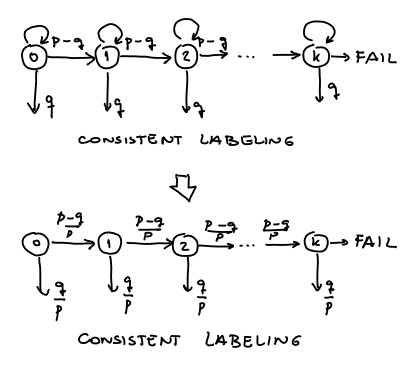
The probability that {S} is consistently labeled is smaller greater than the probability that it is consistently labeled in the same iteration before the set is hit {k} times. In one iteration three things may happen: either the set is not hit, or it is hit but it is not consistently labeled or it is consistently labeled. The figure below measures how many times the set is hit. The down arrows represent the event that the set {S} is consistently labeled:

consist_lab

A standard trick in this cases is to disregard the self-loops and normalize the probabilities. This way the probability that {S} is consistently labeled is:

\displaystyle \frac{q}{p} \sum_{j=0}^{k-1} \left( \frac{p-q}{p} \right)^j = \frac{q}{p} \cdot \frac{ 1 - \left( \frac{p-q}{p} \right)^k }{1 - \frac{p-q}{p} } = 1 - \left( 1 - \frac{q}{p} \right)^k

Now, we just use that {p \leq \frac{k \vert S \vert}{\vert L \vert}} and {q = \frac{z_S}{\vert L \vert}} to obtain the desired result. \Box

The approximation factor of {2 f_{max}} follows straight from the previous theorem by considering the following inequalities:

\displaystyle \left( 1 - \frac{a}{k}\right)^k \leq e^{-a} \leq 1 - \frac{a}{2}

and noting that the LP solution is a lower bound of the optimal value

Theorem 2 The rounding procedure gives a randomized algorithm that, in expectation, achieves a {2 f_{max}} approximation to the optimal consistent labeling.

Sparsest Cut via Metric Embeddings

June 10th, 2009 No comments

A very powerful technique to design approximation algorithms is called metric embeddings. A lot of problems are easy when the graph has some special structure like a tree or a cycle or when the vertices are encoded as points in a {{\mathbb R}^n}. This gives us more structure to the problem an allows us to make geometric considerations about the object we are studying – and this is sometimes the key to find a good approximation. The basic idea is to start with a space without much structure and try to approximate it by some space with stronger geometric or topological properties. A lot has be done recently in finding cuts in graphs or solving Steiner Tree problems.

Consider the problem of finding the sparsest cut in a graph. Given a graph {G = (V,E)}, we define the sparsity of a {(S, \overline{S})} as:

\displaystyle \alpha(S) = \frac{\vert \partial S \vert}{\min\{ \vert S \vert, \vert V \setminus S \vert \}}

where {\partial S } is the set of edges with one endpoint in {S} and other in {\overline{S})}. The sparsest cut is the cut minimizing the sparsity. A related problem is the flux problem, which asks for a cut minimizing:

\displaystyle f(S) = \frac{\vert \partial S \vert}{ \vert S \vert \cdot \vert V \setminus S \vert}

If we can minimize flux, we have a {2}-approximation for sparsity, since for all {S} we have that: {\frac{\alpha(S)}{\vert V \vert} \leq f(S) \leq \frac{2 \alpha(S)}{\vert V \vert}}. If we can approximate the minimum flux, we can also approximate sparsity by the same factor multiplied by {2}.

Let’s formulate flux as an embeddings problem: we would like a mapping {\phi: V \longrightarrow \{0, 1\}} such that minimizes:

\displaystyle \frac{\sum_{(u,v) \in E} \vert \phi(u) - \phi(v) \vert }{ \sum_{(u,v) \in V^2}  \vert \phi(u) - \phi(v) \vert }

Let’s relax this a bit. Substitue {\vert \phi(u) - \phi(v) \vert} by d_{uv}. So, we want to minimize {\frac{\sum_{(u,v) \in E} d_{uv} }{\sum_{(u,v) \in V^2} d_{uv} }}. A standard trick for minimizing fractions where both numerator and denominator are linear functions on the same variables is to fix the denominator to be {1} and minimize the denominator. So, we want to minimize {\sum_{(u,v) \in E} d_{uv}} given that {\sum_{(u,v) \in V^2} d_{uv} = 1}. We also wanted {d_{uv} \in \{ 0, 1\}}. But this is still not enough, we want {d_{uv} } to be of a specific form called cut metric, i.e., there is a partition of {V} in two sets and {d_{uv} = 1} iff {u} and {v} are in different sets. We relax it a bit by just asking it to be a metric, i.e, non-negative value so that the triangle inequality holds:

\displaystyle d_{uv} \leq d_{uw} + d_{wv}

By relaxing a minimization problem we might get a solution which has actually smaller than the previous problem. This gives however a lower bound to the result. In general, finding a good lower bound is the first step in the analysis of approximation algorithms.

Theorem 1 The solution of the flux problem is lower-bounded by the solution of the following LP:

\displaystyle \left. \begin{aligned} & \min \sum_{(u,v) \in E} d_{uv} \text{ s.t. } \\ & \qquad \left\lbrace \begin{aligned} & \sum_{(u,v) \in V^2} d_{uv} = 1 \\ & d_{uv} \leq d_{uw} + d_{wv} \\ & d_{uv} \geq 0 \end{aligned} \right. \end{aligned} \right. \ \ \ \ \ (1)

The idea for approximating this is to drop the integrality constraint, solve the LP to get a general metric and the round it to obtain a cut. Suppose {\{d_{uv}\}} is the optimal solution to the LP version of the program above. How to get a cut from it?

To do it, we will use a powerful result due to Bourgain, but first, let’s discuss some basics about metrics and embeddinds. A metric space is a pair {(X,d)} where {X} is a set and {d:X^2 \longrightarrow {\mathbb R}_+}. Examples of metric spaces are:

  1. {X} is the set of vertices of a weighted graph {G} and {d(u,v)} is the distance from {u} to {v} in the graph;
  2. {X = {\mathbb R}^n} and {d} is the {L_p}-norm, i.e., {d(u,v) = ( \sum_{i=1}^n \vert u_i - v_i \vert^p )^{1/p}}, when {p = 2}, this is the Euclidian norm, when {p = 1}, it is the Manhattan distance. This space is called {L^n_p} ;
  3. {X = {\mathbb R}^n} and {d} is the {L_\infty}-norm, i.e., {d(u,v) = \max_i \vert u_i - v_i \vert}. It is called {L_\infty} norm, because it {\Vert u - v \Vert_\infty = \lim_{p \rightarrow \infty} \Vert u - v \Vert_p} where {\Vert u - v \Vert_p} denoted the distance in the {L_p} norm. This space is called {L^n_\infty}

Given two metric spaces {(X,d_X)} and {(Y, d_Y)}, we say that a mapping {\phi:X \longrightarrow Y} is a distortion {D} embedding:

\displaystyle d_X (u,v) \leq d_Y(\phi(u), \phi(v)) \leq D d_X (u,v)

to make our life easier, we use most of the times the following (not so) weaker definition: we say it is a distortion {D} embedding if there is some factor {\gamma > 0} such that:

\displaystyle \gamma d_X (u,v) \leq d_Y(\phi(u), \phi(v)) \leq D \gamma d_X (u,v)

this is the same but allowing some scaling.

Bourgain’s Theorem says that:

Theorem 2 (Bourgain) For any metric space {(X,d)} with {|X| = n} there is an embedding into {L_1^{O(\log^2 n)}} with distortion {O(\log n)}. And we can construct this embedding in poly-time using a randomized algorithm.

Supose {\phi} is such embedding. Then we have a function {\phi : V \rightarrow {\mathbb R}^{O(log^2 n)}} such that {d_{uv} \leq \Vert \phi(u) - \phi(v) \Vert \leq d_{uv} \cdot O(\log n)}. Now, this gives us {O(n \log^2 n)} cuts obtained in the following way: for each coordinate {i} of {{\mathbb R}^{O(log^2 n)}}, order the {n} points according to {\phi_i(u)} and for each {j = 1 \ldots n-1} take the cut {S} formed by the first {j} points. Let this be the cut {S_{ij}} Then, take the minimum of those cuts.

Theorem 3 The procedure described above generates a cut within a factor of {O(\log n)} to the optimal in poly-time.

To prove this, first we need some notation. Given the cut {(S_{ij}, \overline{S_{ij}})}, let {d_{S_{ij}}} be the cut-distance associated with it, i.e., {d_{S_{ij}} (u,v)} is {0} if {u} and {v} are in the same side of the cut and {1} otherwise. Let also {\{ x_{i1} \leq x_{i1} \leq \ldots \leq x_{in} \} = \{ \phi_i(v); v \in V \}}. It is not difficult to see that:

\displaystyle \vert \phi_i(u) - \phi_i(v) \vert = \sum_{j=1}^{n-1} (x_{i,j+1} - x_{i,j}) d_{S_{ij}} (u,v)

and, therefore:

\displaystyle \Vert \phi(u) - \phi(v) \Vert_1 = \sum_{i=1}^{O(\log^2 n)} \sum_{j=1}^{n-1} (x_{i,j+1} - x_{i,j}) d_{S_{ij}} (u,v)

Now, we can go ahead and prove the theorem: Let {f^*} be the optimal flux and {f} the flux obtained by the algorithm. We have that:

\displaystyle f^* \leq f = \min_{ij} \frac{ \sum_{(u,v)\in E} d_{S_{ij}(u,v)}}{ \sum_{(u,v)\in V^2} d_{S_{ij}(u,v)}} = \min_{ij} \frac{ c_{ij} \sum_{(u,v)\in E} d_{S_{ij}(u,v)}}{ c_{ij} \sum_{(u,v)\in V^2} d_{S_{ij}(u,v)}}

where {c_{ij} = x_{i,j+1} - x_{i,j}}. Then:

\displaystyle f \leq \frac{\sum_{ij} \left[ c_{ij} \sum_{(u,v)\in E} d_{S_{ij}}(u,v) \right] }{\sum_{ij} \left[ c_{ij} \sum_{(u,v)\in V^2} d_{S_{ij}(u,v)} \right] } = \frac{\sum_{(u,v)\in E} \left[ \sum_{ij} c_{ij} d_{S_{ij}}(u,v) \right] }{ \sum_{(u,v)\in V^2} \left[ \sum_{ij} c_{ij} d_{S_{ij}(u,v)} \right] }

but this is exacly the expression of {L_1}-norm, so:

\displaystyle f \leq \frac{\sum_{(u,v)\in E} \Vert \phi(u) - \phi(v) \Vert_1 }{ \sum_{(u,v)\in V^2} \Vert \phi(u) - \phi(v) \Vert_1 } \leq \frac{\sum_{(u,v)\in E} O(\log n) d_{uv} }{ \sum_{(u,v)\in V^2} d_{uv} }

which is smaller than {f^* O(\log n)} since this is the solution to the LP, which is a relaxed version of the original problem. And this finishes the proof.

This is one of the first applications to metric embeddings. It was introduced in a paper by Linal, London and Rabinovich. There are very nice resources on the web about metric embeddins, as the course by Anupam Gupta at CMU, the course by Michael Goemans at MIT and the course by Tim Roughgarden at Stanford.

This is also an area full of exciting open problems. It is known, for example, that it is hard to decide if a given metric is embeddable in {L_1} or not. But given a metric that we know that is isometrically embeddable in {L_1}, how to find the embedding? This is an open problem. In fact, it is unknown even how to approximate this embedding by a factor better then {\log n}, which is given by Bougain’s Theorem.